What the heck is electron spin? (Part 1)
The magnetic moment of an electron resembles what we would expect from a spinning charge, except for a factor of two and a tiny extra correction. Following these discrepancies takes us through the discovery of electron spin, Dirac’s relativistic theory, and one of the most precise tests of quantum electrodynamics.
Originally written in April 2019 for a PHYS 512 (Advanced Quantum Mechanics II) course project during my PhD at the University of Alberta. This is the first of two articles; the second works through Luttinger’s calculation. I used OpenAI’s Codex to adapt my existing writing and research materials into this article and develop the interactive figures and layout.
The gyromagnetic ratio
The word ‘spin’ makes an electron sound like a little ball rotating about an axis. What an electron carries is an intrinsic angular momentum, which we call  . An electron has spin
 : measuring its spin along a chosen direction gives one of two values,
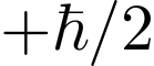 or
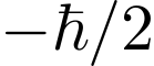 .
To understand why this is a quantum property, it is useful to compare the electron’s magnetic moment with that of a rotating charge. We can then carry the classical result over to electron spin and see where the analogy breaks down.
Consider the classical problem first: a sphere of total mass  , total positive charge
 , and radius
 rotating at constant angular speed
 , with both the mass and charge distributed uniformly within its volume. Moving charge produces a current, giving the sphere a magnetic moment
 . The rotating mass gives it angular momentum
 .
Integrating over the sphere gives the magnitudes of these two quantities:
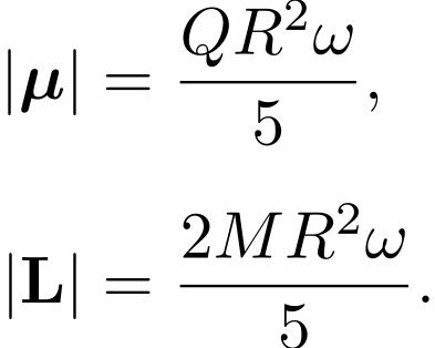
The gyromagnetic ratio,  , is the ratio of the magnetic moment to the angular momentum. For this positively charged sphere,

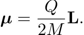
Both moments contain the same factor 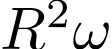 : the radius squared and the angular speed cancel when we take their ratio. The magnetic moment is therefore proportional to the angular momentum,
A uniformly charged sphere

Integrating the rotating mass and charge
The uniform mass and charge densities are

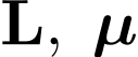
Consider an infinitesimal ring at distance  from the axis. Its period is
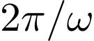 , so its current gives a magnetic moment proportional to its charge, while its angular momentum is proportional to its mass:

Integrating these contributions over the volume gives the expressions above. This comparison assumes the same spatial distribution of charge and mass.
The g-factor of the electron
If we carry the classical relation over to an electron of mass  and charge
 , replacing the orbital angular momentum by the intrinsic spin , we would expect its spin magnetic moment to have the form
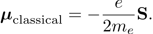
However, spin is not a classical property, and the spin magnetic moment deviates from this result by a factor known as the electron spin g-factor:

Here 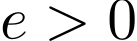 ; the minus sign means that the magnetic moment points opposite to the spin. The form of the relation is the same as for the sphere, but the classical analogy predicts
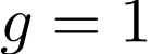 , while the electron has
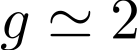 . It is the factor relating angular momentum to magnetic moment that we want to understand.
From spectroscopy to spin
The Zeeman effect, discovered by Dutch physicist Pieter Zeeman in 1896, showed that atomic emission spectra split into multiple lines when influenced by a magnetic field. This proved to be a seminal discovery in the path towards quantum mechanics, though the ordinary effect could be understood through the classical notion of orbital angular momentum.
Thomas Preston subsequently reported splittings that were not explainable through that theory. This effect was named (perhaps unfairly) the ‘anomalous Zeeman effect’, and prompted the idea that electrons had an additional angular momentum, independent from their orbital contribution. [1] [2]
In 1925, with the blessing of their advisor Paul Ehrenfest, George Uhlenbeck and Samuel Goudsmit published a paper that suggested the anomalous Zeeman effect could be explained through the introduction of a new quantum number, implying the existence of electron spin. However, they were not the first to propose this concept. [3]
Arthur Compton had already suggested quantized electron rotation in 1921, though, as Goudsmit later judged, the reasons he had given were unconvincing. A few months prior to the Uhlenbeck and Goudsmit paper, Ralph Kronig (of Kronig–Penney model fame) had performed calculations positing electron spin, but was dissuaded from publishing by Wolfgang Pauli, who criticized the idea because it did not agree with the fine structure of hydrogen. [3]
After warming up to spin, Pauli formulated a phenomenological extension to the Schrödinger equation in 1927, now known as the Pauli–Schrödinger equation. It was within this context that he introduced the ubiquitous Pauli matrices, though the spin degree of freedom and magnetic coupling had to be put in by hand.
It was only with the Dirac equation in 1928 that a fundamental explanation of the factor of two emerged. [4] [5]
The magnetic energy
A magnetic field lets us see what this factor does. The interaction energy is  . For a field pointing along the spin-quantization axis, there are two spin energies, with a splitting proportional to the field:

The constant  is called the Bohr magneton. At a fixed magnetic field, a larger
 means a larger energy difference between the two spin states. These are the spin contributions; orbital motion can contribute to the total energy as well.
The anomalous magnetic moment
Over the next couple of decades the precision of atomic experiments improved greatly, and it became apparent that the Dirac equation’s prediction of the g-factor was not quite complete. The g-factor was slightly more than two. We write this as

The small quantity  is the anomalous magnetic moment. The word ‘anomalous’ here means a departure from the Dirac value. It is a different issue from the older anomalous Zeeman effect that helped motivate electron spin.
As spectroscopic techniques and equipment improved, very precise measurement of the hydrogen ground-state splitting became possible. In 1947, John Nafe and Edward Nelson carried out an atomic-beam measurement of the hyperfine structure of hydrogen, and found a small discrepancy between the theoretical transition frequency and their experimental value. Together with the other precision results of the period, it pointed to a g-factor slightly larger than two. [6]
The results discussed at Shelter Island in June 1947 made this an urgent problem for quantum electrodynamics (QED), the theory of electrons interacting with the electromagnetic field. QED ostensibly should have predicted this departure, but it was beset by infinities that made the first-principles calculation of the g-factor extremely difficult. It was with the development of renormalization that these calculations became possible.
In 1948, with his newly developed techniques of renormalization, Julian Schwinger calculated the leading correction: [7]

Here  is the fine-structure constant, which sets the strength of the electromagnetic interaction. The result gives
 at this order. In
 , the Dirac contribution is one, while the anomalous contribution is only about 0.00116: a correction of roughly one part in 860. At actual scale, it is barely visible. Zoom in below to see just how small it is.
This was a historical step in the establishment of QED as a fundamental description of the physical world. The measured departure from two had become a quantitative prediction of the theory.
How small is the anomalous contribution?
Schwinger’s leading correction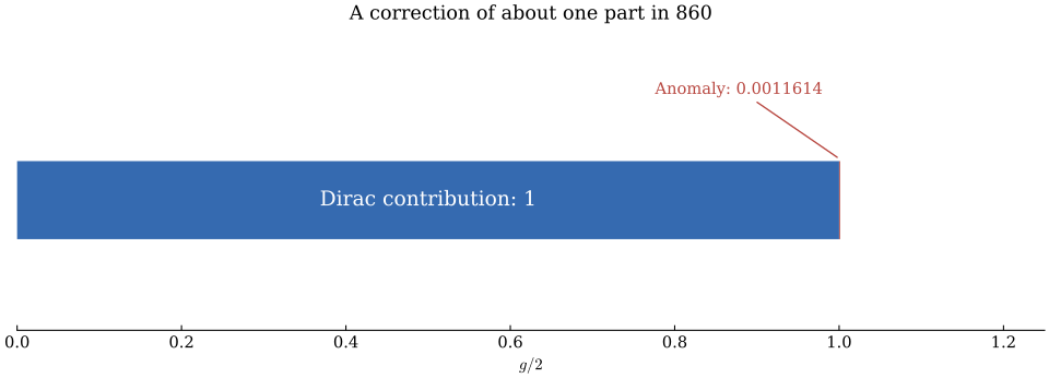
 Dirac contribution

 Anomalous contribution

Blue is the Dirac contribution; red is the extra contribution from the interaction with the electromagnetic field. Both use the same scale, including when you zoom in. This is the leading-order correction, rather than the full modern prediction.
How small a difference can we measure?
As experiments pushed down the uncertainty in the g-factor, higher-order calculations became essential. Schwinger’s expression is the first term of a much longer calculation; it should not be compared with modern measurements as though it were the complete answer.
For example, Fan and collaborators reported a measurement in 2023 of  . Subtracting one gives the anomalous contribution, . The parentheses give the uncertainty in the final digits. [9]
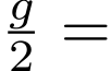
The measurement compares two frequencies of an electron in a magnetic field: a cyclotron frequency,  , associated with its orbital motion, and a spin frequency,
 , associated with flipping its spin. If
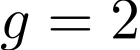 , these frequencies would be equal. Their small fractional difference measures directly:
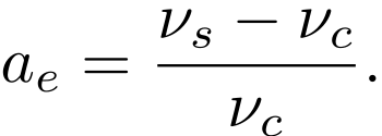
This relation is for a free electron. In the trapped-electron experiment, the measured frequencies must be corrected for the trap and cavity. Comparing the extracted with theory also needs an independent value of ; the 2023 paper discusses the disagreement between independent determinations.
Dodging infinities
Schwinger was not the only person to calculate the leading correction. A few months after his note appeared, Joaquin Luttinger published an alternative derivation. Luttinger is mostly known for his work on Fermi-liquid theory, but here he found an ingenious way of isolating the magnetic response. [10]
His starting point was a special electron state whose orbital and spin magnetic energies cancel. That cancellation turns out to be very useful when the calculation contains an infinite contribution to the mass.
References
- P. Zeeman, The Effect of Magnetisation on the Nature of Light Emitted by a Substance, Nature 55, 347 (1897).
- D. Weaire and S. O’Connor, Unfulfilled renown: Thomas Preston (1860–1900) and the anomalous Zeeman effect, Annals of Science 44, 617–644 (1987).
- S. A. Goudsmit, The discovery of the electron spin, 1971 lecture; English translation by J. H. van der Waals, hosted by the Instituut-Lorentz. Includes the Thomas letter of 25 March 1926.
- W. Pauli, Zur Quantenmechanik des magnetischen Elektrons, Zeitschrift für Physik 43, 601–623 (1927).
- P. A. M. Dirac, The Quantum Theory of the Electron, Proceedings of the Royal Society A 117, 610–624 (1928).
- J. E. Nafe and E. B. Nelson, The Hyperfine Structure of Hydrogen and Deuterium, Physical Review 73, 718–728 (1948).
- J. Schwinger, On Quantum-Electrodynamics and the Magnetic Moment of the Electron, Physical Review 73, 416–417 (1948).
- J. Schwinger, The Greening of Quantum Field Theory: George and I, lecture at Nottingham, 14 July 1993; arXiv:hep-ph/9310283. Reprinted in Julian Schwinger: The Physicist, the Teacher, and the Man (1996).
- X. Fan, T. G. Myers, B. A. D. Sukra and G. Gabrielse, Measurement of the Electron Magnetic Moment, Physical Review Letters 130, 071801 (2023). Open preprint.
- J. M. Luttinger, A Note on the Magnetic Moment of the Electron, Physical Review 74, 893–898 (1948).