Dodging infinities with Luttinger (Part 2)
Calculating the electron’s anomalous magnetic moment brings us face to face with the infinities of quantum electrodynamics. Luttinger found an ingenious shortcut: choose a state whose ordinary orbital and spin magnetic energies cancel, then isolate the small magnetic response left by interactions. Here we follow that calculation and see why his choice of state makes it work.
Originally written in April 2019 for a PHYS 512 (Advanced Quantum Mechanics II) course project during my PhD at the University of Alberta. This companion assumes some familiarity with the Dirac equation and perturbation theory; part 1 introduces the magnetic moment and g-factor. I used OpenAI’s Codex to adapt my existing writing and research materials into this article and develop the interactive figures and layout.
Dodging infinities
As mentioned in the first article, Julian Schwinger was the first to calculate the leading anomalous magnetic moment of the electron. His brief 1948 note gave the result, but little mathematical detail. Later that year, Joaquin Luttinger published his own calculation, showing that the change in magnetic moment could be obtained without an elaborate subtraction formalism. [1] [2]
Luttinger’s method had the advantage of knowing that the QED divergences could be associated with changes in the electron’s mass and charge. His insight was to realize that the lowest positive-energy state of the Dirac electron in a homogeneous magnetic field, with no momentum along the field, has an energy equal to its rest energy. It does not depend on the applied magnetic field.
This is a special case where the orbital and spin magnetic energies cancel. Therefore, when we calculate the energy correction, the field-independent mass contribution can be separated from the term linear in the field. That linear term gives the anomalous magnetic response.
The special Landau level
In a uniform magnetic field, the electron’s motion perpendicular to the field becomes a harmonic-oscillator problem. Its quantized orbital energies are the Landau levels. The spin contributes another magnetic energy. We want the state in which these two energies cancel.
The schematic below shows a lowest-orbital probability cloud in the plane perpendicular to the field. The ladder starts with the orbital energies alone. Add the spin energy, then reverse the spin to see why its orientation matters.
An electron in a uniform field
Dirac prediction ·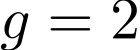
The real-space picture
The magnetic energy ladder

The ladder shows the orbital contribution alone. Add the spin energy to see the total.



Now put this cancellation into equations. Take an electron of charge  in
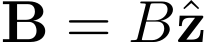 , with no momentum along the field,
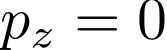 . In the weak-field limit its energy above the rest energy is [3]

Here  labels the orbital state,
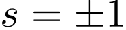 labels the spin direction, and
 is the Bohr magneton. Choose the lowest orbital state and spin down:
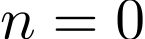 ,
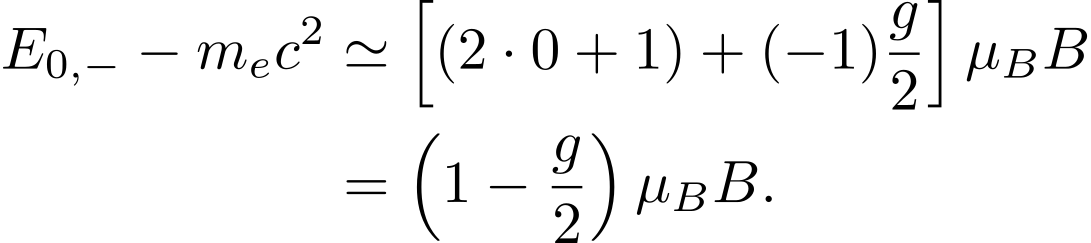
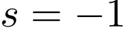 . Substituting those numbers gives
First use the Dirac value
Set . The orbital energy and spin energy are equal and opposite:

Then include the anomalous moment
Write  , so that
 . The orbital term stays the same; the spin term becomes slightly more negative:

The ordinary contributions still cancel. The small energy left over is entirely the anomalous contribution. This is why Luttinger chose this state: calculating the coefficient of its energy shift linear in  tells us
 .
Keep the lowest state selected below, then include the anomalous moment. The numerical readout shows the small remainder.
The anomalous energy shift
Weak field ·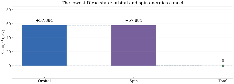




The sum

The spin column starts where the orbital column ends; the total is measured from zero. Blue adds the orbital energy, purple adds the spin energy, and green shows the sum. With the anomalous moment included, its extra contribution is red. Its size is given numerically because it is barely visible at this scale.
The exact Dirac spectrum and its lowest state
The positive-energy solutions of the minimally coupled Dirac equation satisfy

For , and , the factor  . The positive-energy state therefore has
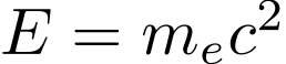 exactly, before any weak-field expansion. [3]
For an electron of charge , define the kinetic momentum  . Squaring the minimally coupled Dirac Hamiltonian separates the orbital and spin terms:

The eigenvalues of  are
 , and
 has eigenvalues . Substituting these gives the spectrum above. With and , the two magnetic terms cancel before any weak-field expansion is made.
Does relativity alone force the g-factor to be two?
Though the minimally coupled Dirac equation provides a fundamental derivation, there remains a question whether it is possible to add a term that modifies the g-factor. Weinberg observed that an additional Pauli term is compatible with Lorentz and gauge invariance. The important qualification is minimal coupling: interaction effects can produce an effective Pauli coupling, whose coefficient describes the anomalous magnetic moment. [4]
What we need from the calculation
The special state has no ordinary magnetic energy when . Interactions can shift its energy, but we only need the part that changes linearly with the applied magnetic field. Write the correction as

The constant contains the divergent mass contribution. It shifts the rest energy but does not change the slope with respect to . The finite coefficient  gives the magnetic response. Comparing with the lowest-state result above,

The task is now to calculate one coefficient, . The minus sign matters: a positive anomaly lowers the energy of this spin-down state.
The magnetic response as an energy derivative
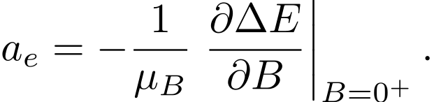
This is the same coefficient-matching argument written as a derivative at vanishing applied field.
Calculating the energy shift
We know which state to use and which coefficient to extract. We next calculate how that state’s energy changes when the electron interacts with the electromagnetic field.
1. Identify the interactions
Separate the applied magnetic field from the dynamical radiation field, which supplies the photons. The Hamiltonian has three parts:


- The Dirac electron in the applied field, plus the free radiation field. We have already solved this part by choosing the lowest Landau state.
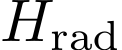
- The interaction between the electron current and the radiation field.

- The Coulomb interaction between charge densities.
Our reference state  contains one electron in the special lowest level and no photons, along with the filled negative-energy states of the historical hole-theory formulation. We compare its energy with that of the vacuum, which has no additional electron.
2. Find the interaction energy
The radiation interaction creates or annihilates a photon. Acting once on a no-photon state cannot return it to itself, so its first-order expectation value is zero. At second order, a virtual intermediate state can contribute: a photon can be created and then absorbed. The Coulomb term already has a nonzero first-order expectation value. Both contributions enter at order  .
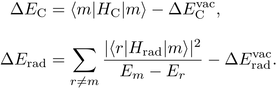
The first line is the direct expectation value of the Coulomb interaction. The second adds the allowed intermediate states  , weighted by their matrix elements and energy denominators. The superscript “vac” means the corresponding correction calculated for the vacuum. Subtracting the vacuum contribution leaves the energy cost of adding the electron.
The orbital state and intermediate states
In the gauge  , a guiding-centre eigenstate has a Gaussian transverse wavefunction:

The real-space schematic shows a localized lowest-Landau orbital, obtained by combining the degenerate guiding-centre states. It illustrates the probability distribution rather than a classical electron trajectory. The energy calculation sums over the complete Dirac–Landau basis, including the positive- and negative-energy solutions, and over the photon states. Luttinger’s paper gives the matrix elements, sums and momentum integrals. [2]
3. Keep the term linear in the field
The applied field was included in from the start. We first expand in the interactions; we then expand the resulting correction in the applied field strength. These are two distinct expansions.
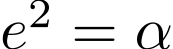
In his Gaussian natural-unit convention,  and
 . The results for the static Coulomb and dynamical radiation contributions are
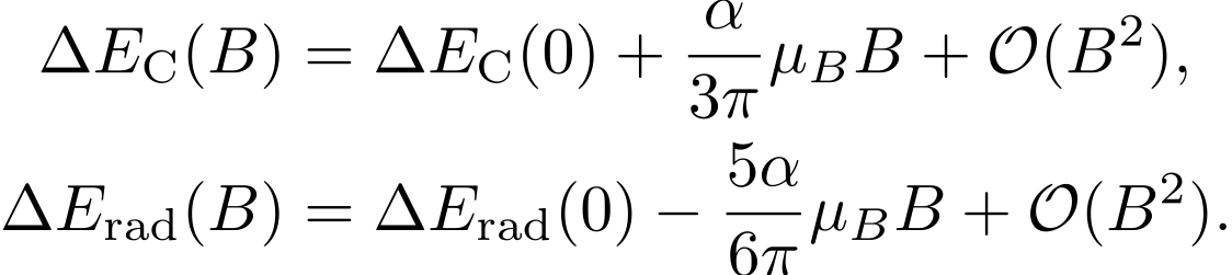
The terms at 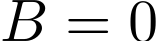 contain the remaining electron self-energy divergence. Subtracting the vacuum has not removed it; it is absorbed into the measured mass. We do not need its value to add the two finite coefficients of :

This finite coefficient is the result we needed. Multiplying by gives the small field-dependent energy left after the ordinary orbital and spin contributions cancel.
Extracting the anomalous moment
Now match the calculated coefficient to the lowest-state energy. The anomalous moment gives a shift linear in the field, so
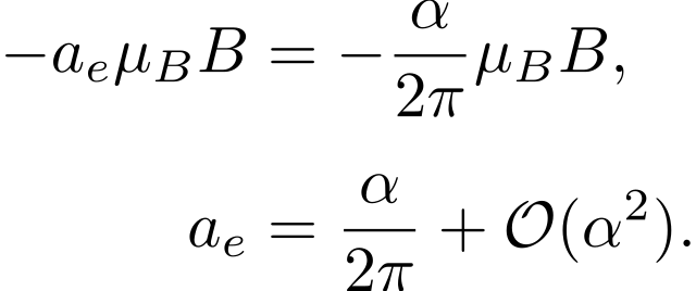
The common factor 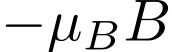 cancels. Thus gives

Luttinger obtains the same leading result as Schwinger. Though a historical footnote beside Schwinger’s work, his calculation is an ingenious workaround to a problem that had stymied physicists: the special choice of state lets the finite magnetic response be separated from the divergent mass contribution.
The calculation of the anomalous spin magnetic moment by Schwinger remains one of the crowning achievements of theoretical physics, nearly eight decades since its publication. Although Feynman diagrams became the standard language for organizing perturbative calculations, the elegance of Schwinger’s proper-time formulation and his use of Green’s functions remain powerful examples of solving gauge-theory problems in a gauge-invariant manner.
In 1993, Julian Schwinger gave a lecture in Nottingham, expounding on the life of George Green and the effect that Green’s functions had on his own work. He ended this lecture with the words:
“What, finally, shall we say about George Green? Why, that he is, in a manner of speaking, alive, well, and living among us.” [7]
Given Julian Schwinger’s contributions to the field of theoretical physics—with his methods still serving as a touchstone to physicists around the world—it would only be appropriate to lean upon his work once more: What, finally, shall we say about Julian Schwinger? Why, that he is, in a manner of speaking, alive, well, and living among us.
References
- J. Schwinger, On Quantum-Electrodynamics and the Magnetic Moment of the Electron, Physical Review 73, 416–417 (1948).
- J. M. Luttinger, A Note on the Magnetic Moment of the Electron, Physical Review 74, 893–898 (1948), especially Eqs. (8)–(12) and the appendix.
- K. Bhattacharya, Solution of the Dirac equation in presence of an uniform magnetic field (2007), for the Landau-state conventions.
- S. Weinberg, The Quantum Theory of Fields, Volume I, chapter 1, discussion of the magnetic moment and the Pauli coupling.
- S.-I. Tomonaga, Development of Quantum Electrodynamics, Nobel lecture, 6 May 1966 (1965 Nobel Prize).
- P. A. M. Dirac, Lectures (1956), Lindau Mediatheque, transcript of the negative-energy-state discussion.
- J. Schwinger, The Greening of Quantum Field Theory: George and I, lecture at Nottingham, 14 July 1993; arXiv:hep-ph/9310283.
- J. Schwinger, On Gauge Invariance and Vacuum Polarization, Physical Review 82, 664–679 (1951).